Lead Evolution Geom for Stacey & Kramers (1975)
Source:R/ASTR_geom_stacey_karmers.R
geom_sk_lines.RdThese Geoms draws and label isochron, geochron, and kappa lines used for isotope age model referencing in lead isotope biplots. The lines follows the model used by Stacey & Kramers (1975).
Usage
geom_sk_lines(
  mapping = NULL,
  data = NULL,
  system = c("76", "86"),
  Mu1 = 10,
  Kappa = 4,
  ...
)

geom_sk_labels(
  mapping = NULL,
  data = NULL,
  system = "76",
  Mu1 = 10,
  Kappa = 4,
  ...
)
Arguments
- mapping
Set of aesthetic mappings created by
aes(). If specified andinherit.aes = TRUE(the default), it is combined with the default mapping at the top level of the plot. You must supplymappingif there is no plot mapping.- data
The data to be displayed in this layer. There are three options:
If
NULL, the default, the data is inherited from the plot data as specified in the call toggplot().A
data.frame, or other object, will override the plot data. All objects will be fortified to produce a data frame. Seefortify()for which variables will be created.A
functionwill be called with a single argument, the plot data. The return value must be adata.frame, and will be used as the layer data. Afunctioncan be created from aformula(e.g.~ head(.x, 10)).- system
Character "76" or "86" defining the isotope plot axis (default "76").
- Mu1
Second-stage 238U/204Pb ratio (default 10).
- Kappa
Second-stage 232Th/238U ratio (default 4).
- ...
Additional parameters for the geoms (see Details) and other arguments passed on to
ggplot2::layer(). These are often aesthetics used to set a fixed value, such ascolour = "red"oralpha = 0.5.
Details
The plotting system follows the convention of showing geochron and isochron lines for the 207Pb/204Pb vs. 206Pb/204Pb plot and the kappa lines for 208Pb/204Pb vs. 206Pb/204Pb plot.
The geoms accept the following additional parameters through ...:
Ti: Initial time of the second stage in years (default 3.7 Ga).interval: Time interval for isochron labels in years (default 200 Ma).show_geochron: Logical; should the Geochron be plotted? (defaultTRUE).show_isochrons: Logical; should time isochrons be plotted? (defaultTRUE)kappa_list: Numeric vector of Kappa values to plot in "86" system.
Note
Currently the plot will scale the xlim and ylim to their maximum bounds. To
prevent this, use coord_cartesian(xlim, ylim)
to force the axis range to the desired values.
Aesthetics
geom_sk_lines() and geom_sk_labels() accept the
following aesthetic values:
alphacolour(controls the polygon outline)fill(controls the polygon fill)linetypelinewidth(controls the outline thickness)text.colour(controls colour of the text)size.unit(controls size aesthetic in "mm", "pt", "cm", "in" or "pc")Learn more about setting these aesthetics in
vignette("ggplot2-specs").
References
Stacey, J.S. and Kramers, J.D. (1975) Approximation of terrestrial lead isotope evolution by a two-stage model. Earth and Planetary Science Letters 26(2), pp. 207–221. https://dx.doi.org/10.1016/0012-821X(75)90088-6.
See also
Other Pb isotope functions:
age_models
Examples
# example code
library(ggplot2)
set.seed(50)
df <- data.frame(
pb64 = rnorm(10, 18,0.2),
pb74 = rnorm(10, 15.7,0.1),
pb84 = rnorm(10, 37.5,0.1)
)
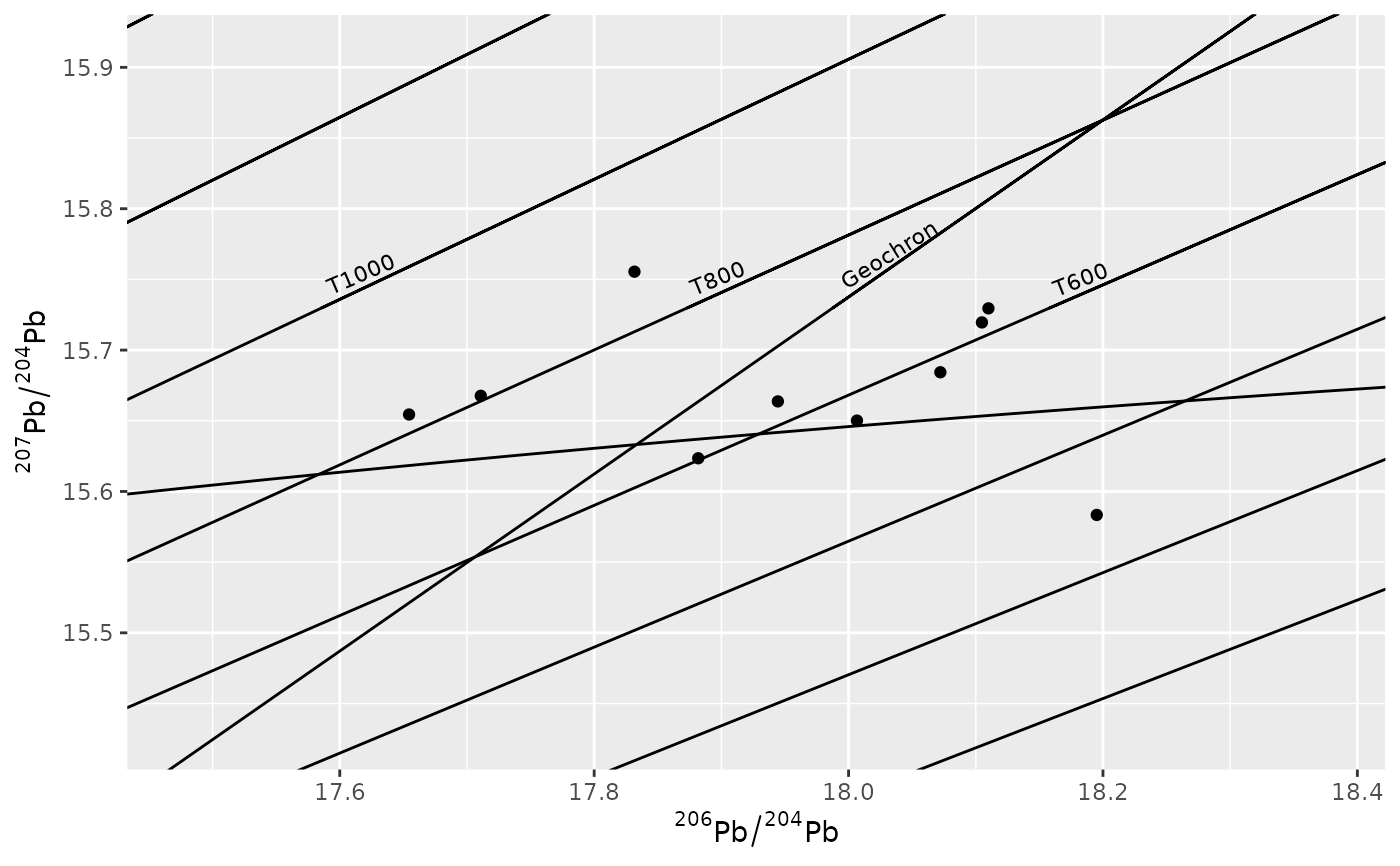
# Creating the Pb 207/204~206/204 plot
ggplot(df, aes(x = pb64, y = pb74)) +
geom_point() +
geom_sk_lines(system = "76") +
geom_sk_labels(system = "76") +
coord_cartesian(
xlim = range(df$pb64) * c(.99, 1.01),
ylim = range(df$pb74) * c(.99, 1.01)
) +
labs(
x = expression({}^206*Pb / {}^204*Pb),
y = expression({}^207*Pb / {}^204*Pb),
)
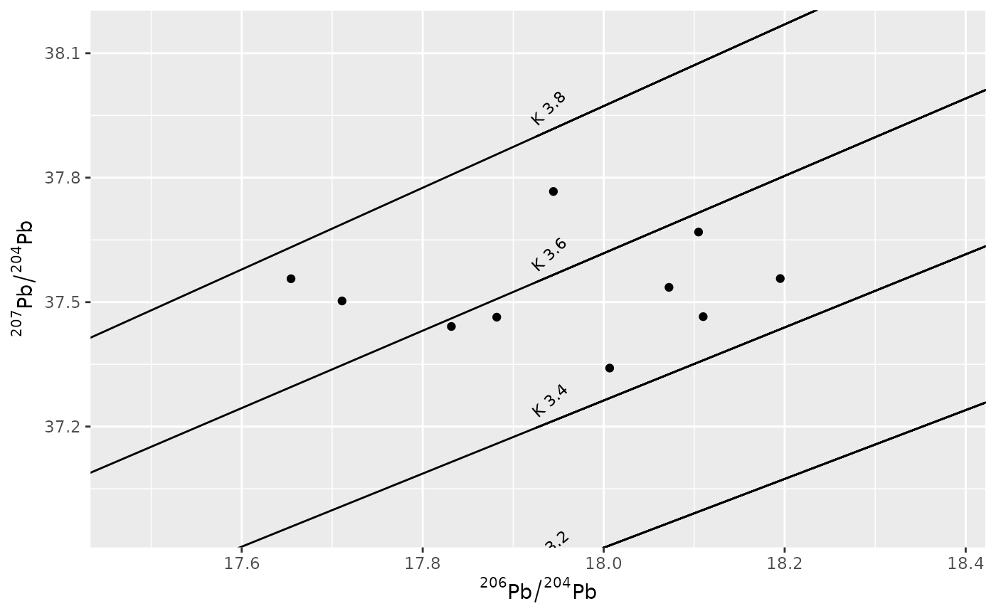
 # Creating the Pb 208/204~206/204 plot
ggplot(df, aes(x = pb64, y = pb84)) +
geom_point() +
geom_sk_lines(system = "86",
show_isochrons = FALSE, show_geochron = FALSE,
kappa_list = c(3.2, 3.4, 3.6, 3.8)) +
geom_sk_labels(system = "86",
show_isochrons = FALSE, show_geochron = FALSE,
kappa_list = c(3.2, 3.4, 3.6, 3.8)) +
coord_cartesian(
xlim = range(df$pb64) * c(.99, 1.01),
ylim = range(df$pb84) * c(.99, 1.01)
) +
labs(
x = expression({}^206*Pb / {}^204*Pb),
y = expression({}^207*Pb / {}^204*Pb),
)
# Creating the Pb 208/204~206/204 plot
ggplot(df, aes(x = pb64, y = pb84)) +
geom_point() +
geom_sk_lines(system = "86",
show_isochrons = FALSE, show_geochron = FALSE,
kappa_list = c(3.2, 3.4, 3.6, 3.8)) +
geom_sk_labels(system = "86",
show_isochrons = FALSE, show_geochron = FALSE,
kappa_list = c(3.2, 3.4, 3.6, 3.8)) +
coord_cartesian(
xlim = range(df$pb64) * c(.99, 1.01),
ylim = range(df$pb84) * c(.99, 1.01)
) +
labs(
x = expression({}^206*Pb / {}^204*Pb),
y = expression({}^207*Pb / {}^204*Pb),
)
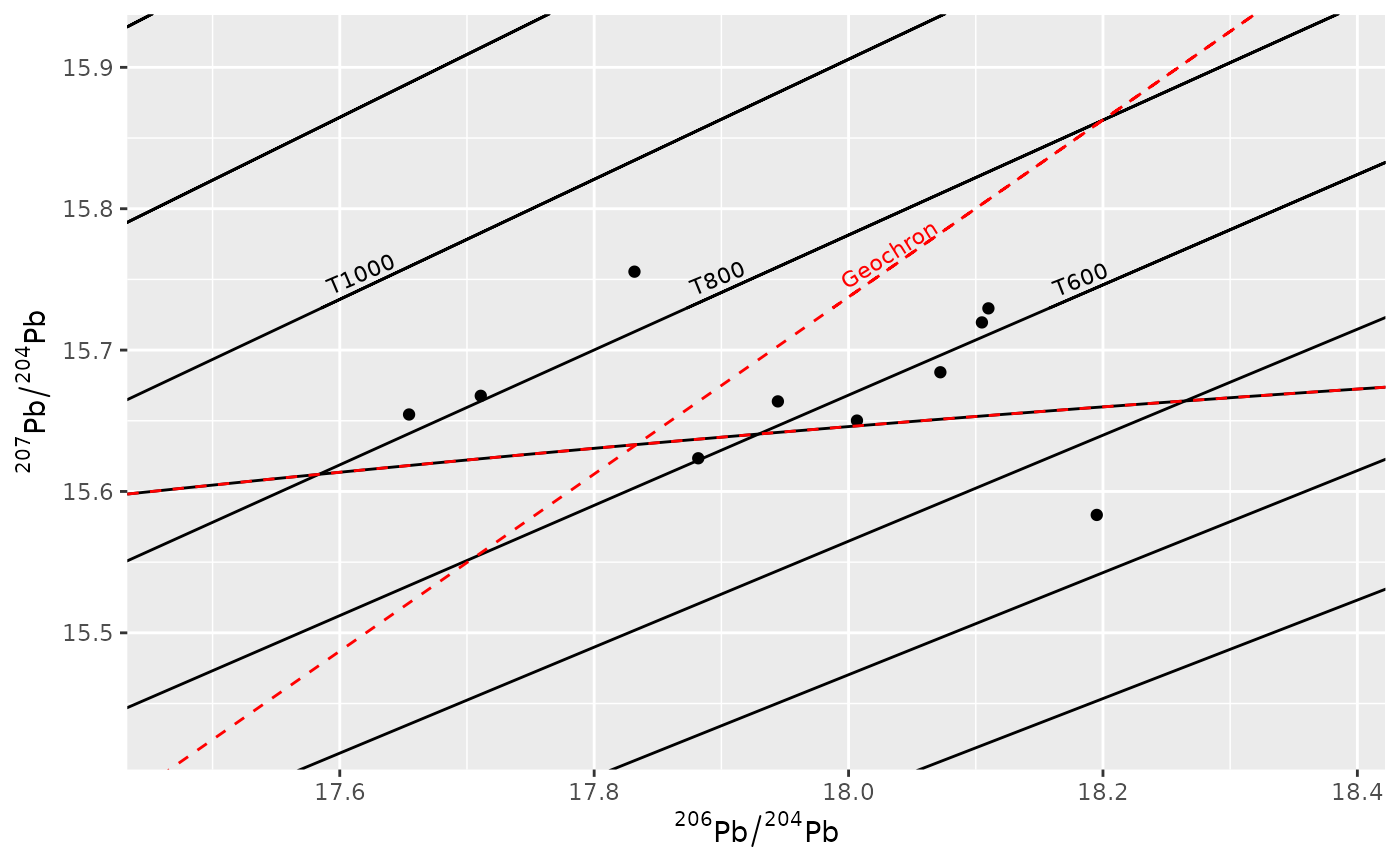
 # Creating the Pb 207/204~206/204 plot with a seperate Geocrone color
ggplot(df, aes(x = pb64, y = pb74)) +
geom_point() +
geom_sk_lines(system = "76", show_geochron = FALSE) +
geom_sk_lines(system = "76", show_isochrons = FALSE,
color = 'red', linetype = 'dashed') +
geom_sk_labels(system = "76", show_geochron = FALSE) +
geom_sk_labels(system = "76", show_isochrons = FALSE, color = 'red') +
coord_cartesian(
xlim = range(df$pb64) * c(.99, 1.01),
ylim = range(df$pb74) * c(.99, 1.01)
) +
labs(
x = expression({}^206*Pb / {}^204*Pb),
y = expression({}^207*Pb / {}^204*Pb),
)
# Creating the Pb 207/204~206/204 plot with a seperate Geocrone color
ggplot(df, aes(x = pb64, y = pb74)) +
geom_point() +
geom_sk_lines(system = "76", show_geochron = FALSE) +
geom_sk_lines(system = "76", show_isochrons = FALSE,
color = 'red', linetype = 'dashed') +
geom_sk_labels(system = "76", show_geochron = FALSE) +
geom_sk_labels(system = "76", show_isochrons = FALSE, color = 'red') +
coord_cartesian(
xlim = range(df$pb64) * c(.99, 1.01),
ylim = range(df$pb74) * c(.99, 1.01)
) +
labs(
x = expression({}^206*Pb / {}^204*Pb),
y = expression({}^207*Pb / {}^204*Pb),
)