Binary plot with kernel density estimation • ASTR

library(ASTR)

Introduction

This vignette introduces geom_kde2(), which generates a binary plot with kernel density estimation.

Kernel density estimation (KDE) is a non-parametric method to transform continuous data into a smoothed probability density function. According to Y.-K. Hsu (2023) and Y.-K. Hsu et al. (2018), KDE has become popular in archaeological science publications (Pollard et al., 2023) mainly due to three advantages when analysing data:

They do not assume the normality of the data;
They can produce smoother distributions than conventional histograms, whose appearance is significantly affected by the choices of bin width and the start/end points of bins; and
They can represent data in a multidimensional space and enable users to effectively compare different datasets either graphically or mathematically (see also De Ceuster et al. (2025) for the advantages of the use of one-dimensional KDE’s).

What is Kernel density estimation (KDE)?

Kernel density estimation is a widely-used tool for visualising the distribution of data (Simonoff, 1996).

Probability density function (pdf) shows how the whole 100% probability mass is distributed over the x-axis, i.e., over the values of an X random variable. Kernel estimation of probability density function produces a smooth empirical pdf based on individual locations of all sample data. Such pdf estimate seems to better represent the “true” pdf of a continuous variable (Węglarczyk, Stanisław, 2018).

Kernel density estimation calculation

Let the series $\{x_1, x_2, \ldots, x_n\}$ be an independent and identically distributed (i.i.d.) sample of $n$ observations taken from a population $X$ with an unknown probability distribution function $f(x)$ .

The kernel estimate $\hat{f}(x)$ of the original $f(x)$ assigns each $i$ -th sample data point $x_i$ a function $K(x_i, t)$ , called a kernel function, in the following way:

$\hat{f}(t) = \frac{1}{n} \sum_{i=1}^{n} K(x_i, t) \tag{1}$

The kernel function $K(x, t)$ is non-negative and bounded for all $x$ and $t$ :

$0 \leq K(x, t) < \infty \quad \text{for all real } x, t \tag{2}$

and, for all real $x$ ,

$\int_{-\infty}^{\infty} K(x, t) \, dt = 1. \tag{3}$

Property (3) ensures the required normalisation of the kernel density estimate given in (1):

$\int_{-\infty}^{\infty} \hat{f}(t) \, dt = \frac{1}{n} \sum_{i=1}^{n} \int_{-\infty}^{\infty} K(x_i, t) \, dt = 1. \tag{4}$

In other words, the kernel transforms the “sharp” (point) location of $x_i$ into an interval centred (symmetrically or not) around $x_i$ (Węglarczyk, Stanisław, 2018).

Function workflow

geom_kde2() calculates the 2D kernel density estimate using kde() from the ks package (Duong, 2007, 2025), while handling the contours manually (compute.cont = FALSE). It then calculates the actual density values (the contour levels) corresponding to the probability levels (probs) using ks::contourLevels().

Using the base R function grDevices::contourLines(), the contour line coordinates are generated, using the grid points (eval.points) and the density estimate (estimate) from the kde object, and the calculated levels. The contour coordinates are converted into a data frame as list items. The function extracts its coordinates (x, y) and assigns a unique group ID for each contour. Specific error messages are printed for failed density calculations.

The original data are then returned with the added type column and are checked for fallback (values in the type column equals to “points”) to determine if the density estimates failed. A data frame for plotting points using the original x and y data from the fallback data is created, applying the determined aesthetics and these are drawn using the in-built GeomPoint draw_panel.

Default aesthetic values are applied if unchanged by the user.

Examples

The following examples showcase the different visualisation and density estimate calculations for geom_kde2d().

Basic biplot

# load example lead isotope data that is included with the package
data(ArgentinaDatabase)

library(ggplot2)

ggplot(
  ArgentinaDatabase,
  aes(
    x = `206Pb/204Pb`,
    y = `207Pb/204Pb`,
    fill = `Mining site`
  )
) +
  geom_kde2d() +
  theme_minimal() +
  # move the legend under the plot so the
  # site names are fully legible
  theme(
    legend.position = "bottom",
    legend.direction = "horizontal"
  ) +
  guides(fill = guide_legend(
    nrow = 10,
    theme = theme(legend.byrow = TRUE)
  ))
#> No density estimate possible for group '2', plotting points instead: infinite or missing values in 'x'
#> No density estimate possible for group '3', plotting points instead: the leading minor of order 2 is not positive
#> No density estimate possible for group '5', plotting points instead: infinite or missing values in 'x'
#> No density estimate possible for group '12', plotting points instead: infinite or missing values in 'x'
#> No density estimate possible for group '13', plotting points instead: infinite or missing values in 'x'
#> No density estimate possible for group '14', plotting points instead: infinite or missing values in 'x'
#> No density estimate possible for group '16', plotting points instead: infinite or missing values in 'x'
#> No density estimate possible for group '21', plotting points instead: the leading minor of order 2 is not positive
#> No density estimate possible for group '23', plotting points instead: infinite or missing values in 'x'
#> No density estimate possible for group '24', plotting points instead: infinite or missing values in 'x'
#> No density estimate possible for group '25', plotting points instead: infinite or missing values in 'x'

This example reads in the sample dataset and calculates the kernel density estimates in the function geom_kde2d(), colouring by the Mining site variable from the dataset. Warning messages appear for each group where the sample size is too small to calculate the estimates: No density estimate possible for group 'x', plotting points instead: the leading minor of order 1 is not positive. In those cases, the plotting falls back to plotting individual points from the original dataset.

Biplot with adjusted quantiles to show deciles

The default function reverts to 4 quantiles. This examples illustrates the quantiles set to 10 to show deciles. It also sets the transparency to 0.5 (alpha).

ggplot(
  ArgentinaDatabase,
  aes(
    x = `206Pb/204Pb`,
    y = `207Pb/204Pb`,
    fill = `Mining site`
  )
) +
  geom_kde2d(
    quantiles = 10,
    alpha = 0.5
  ) +
  theme_minimal() +
  # move the legend under the plot so the
  # site names are fully legible
  theme(
    legend.position = "bottom",
    legend.direction = "horizontal"
  ) +
  guides(fill = guide_legend(
    nrow = 10,
    theme = theme(legend.byrow = TRUE)
  ))
#> No density estimate possible for group '2', plotting points instead: infinite or missing values in 'x'
#> No density estimate possible for group '3', plotting points instead: the leading minor of order 2 is not positive
#> No density estimate possible for group '5', plotting points instead: infinite or missing values in 'x'
#> No density estimate possible for group '12', plotting points instead: infinite or missing values in 'x'
#> No density estimate possible for group '13', plotting points instead: infinite or missing values in 'x'
#> No density estimate possible for group '14', plotting points instead: infinite or missing values in 'x'
#> No density estimate possible for group '16', plotting points instead: infinite or missing values in 'x'
#> No density estimate possible for group '21', plotting points instead: the leading minor of order 2 is not positive
#> No density estimate possible for group '23', plotting points instead: infinite or missing values in 'x'
#> No density estimate possible for group '24', plotting points instead: infinite or missing values in 'x'
#> No density estimate possible for group '25', plotting points instead: infinite or missing values in 'x'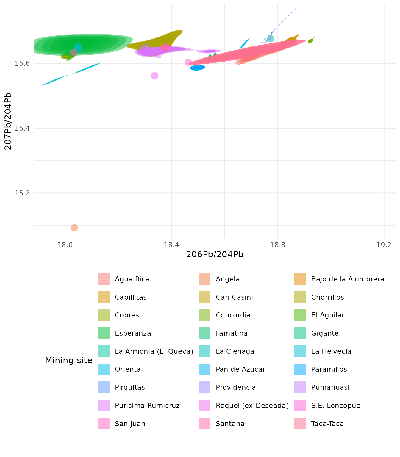

Biplot with the minimum probability argument added to show only density regions above the median

ggplot(
  ArgentinaDatabase,
  aes(
    x = `206Pb/204Pb`,
    y = `207Pb/204Pb`,
    fill = `Mining site`
  )
) +
  geom_kde2d(
    quantiles = 10,
    min_prob = 0.5
  ) +
  theme_minimal() +
  # move the legend under the plot so the
  # site names are fully legible
  theme(
    legend.position = "bottom",
    legend.direction = "horizontal"
  ) +
  guides(fill = guide_legend(
    nrow = 10,
    theme = theme(legend.byrow = TRUE)
  ))
#> No density estimate possible for group '2', plotting points instead: infinite or missing values in 'x'
#> No density estimate possible for group '3', plotting points instead: the leading minor of order 2 is not positive
#> No density estimate possible for group '5', plotting points instead: infinite or missing values in 'x'
#> No density estimate possible for group '12', plotting points instead: infinite or missing values in 'x'
#> No density estimate possible for group '13', plotting points instead: infinite or missing values in 'x'
#> No density estimate possible for group '14', plotting points instead: infinite or missing values in 'x'
#> No density estimate possible for group '16', plotting points instead: infinite or missing values in 'x'
#> No density estimate possible for group '21', plotting points instead: the leading minor of order 2 is not positive
#> No density estimate possible for group '23', plotting points instead: infinite or missing values in 'x'
#> No density estimate possible for group '24', plotting points instead: infinite or missing values in 'x'
#> No density estimate possible for group '25', plotting points instead: infinite or missing values in 'x'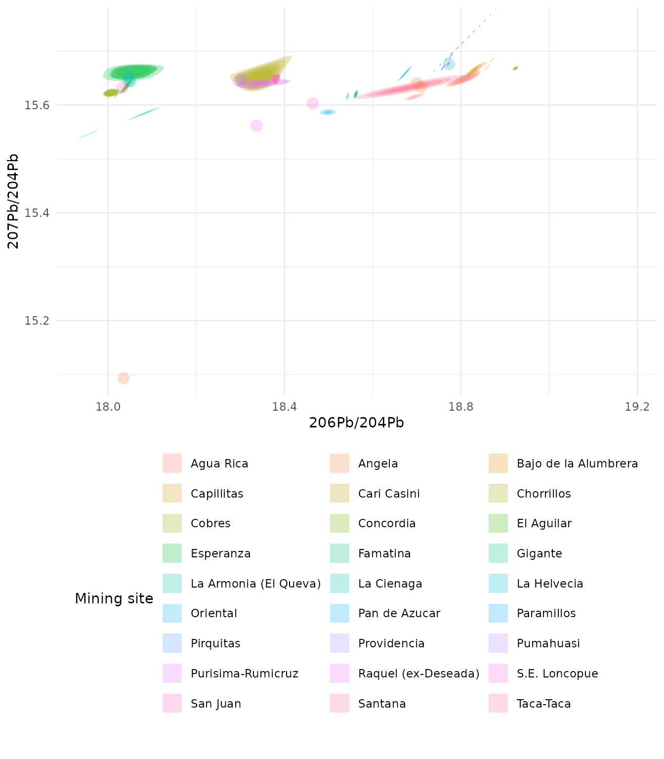

Creation of an outline effect around the density region

For this effect the fill argument is set to NA

ggplot(
  ArgentinaDatabase,
  aes(
    x = `206Pb/204Pb`,
    y = `207Pb/204Pb`,
    colour = `Mining site`
  )
) +
  geom_kde2d(
    quantiles = 1,
    min_prob = 0,
    fill = NA
  ) +
  theme_minimal() +
  # move the legend under the plot so the
  # site names are fully legible
  theme(
    legend.position = "bottom",
    legend.direction = "horizontal"
  ) +
  guides(colour = guide_legend(
    nrow = 10,
    theme = theme(legend.byrow = TRUE)
  ))
#> No density estimate possible for group '2', plotting points instead: infinite or missing values in 'x'
#> No density estimate possible for group '3', plotting points instead: the leading minor of order 2 is not positive
#> No density estimate possible for group '5', plotting points instead: infinite or missing values in 'x'
#> No density estimate possible for group '12', plotting points instead: infinite or missing values in 'x'
#> No density estimate possible for group '13', plotting points instead: infinite or missing values in 'x'
#> No density estimate possible for group '14', plotting points instead: infinite or missing values in 'x'
#> No density estimate possible for group '16', plotting points instead: infinite or missing values in 'x'
#> No density estimate possible for group '21', plotting points instead: the leading minor of order 2 is not positive
#> No density estimate possible for group '23', plotting points instead: infinite or missing values in 'x'
#> No density estimate possible for group '24', plotting points instead: infinite or missing values in 'x'
#> No density estimate possible for group '25', plotting points instead: infinite or missing values in 'x'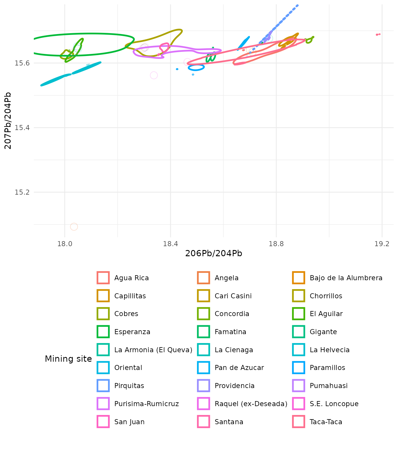

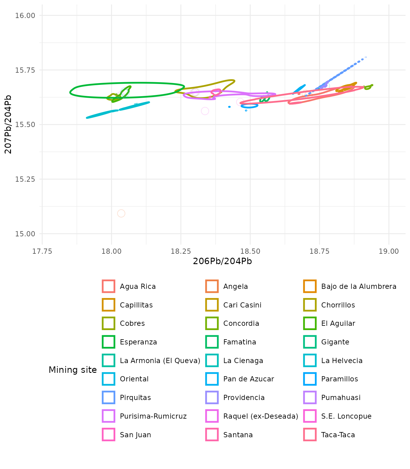
Creation of an outline effect around the density region solving clipping issues

In some cases density regions can be clipped by the plot area. The addition of coord_cartesian() from the package ggplot2 expands the plot area so that the full density regions are shown without clipping. The limits are set for the axes using the xlim and ylim arguments.

ggplot(
  ArgentinaDatabase,
  aes(
    x = `206Pb/204Pb`,
    y = `207Pb/204Pb`,
    colour = `Mining site`
  )
) +
  geom_kde2d(
    quantiles = 1,
    min_prob = 0,
    fill = NA
  ) +
  coord_cartesian(
    xlim = c(17.8, 19),
    ylim = c(15, 16),
    clip = "off"
  ) +
  theme_minimal() +
  # move the legend under the plot so the
  # site names are fully legible
  theme(
    legend.position = "bottom",
    legend.direction = "horizontal"
  ) +
  guides(colour = guide_legend(
    nrow = 10,
    theme = theme(legend.byrow = TRUE)
  ))
#> No density estimate possible for group '2', plotting points instead: infinite or missing values in 'x'
#> No density estimate possible for group '3', plotting points instead: the leading minor of order 2 is not positive
#> No density estimate possible for group '5', plotting points instead: infinite or missing values in 'x'
#> No density estimate possible for group '12', plotting points instead: infinite or missing values in 'x'
#> No density estimate possible for group '13', plotting points instead: infinite or missing values in 'x'
#> No density estimate possible for group '14', plotting points instead: infinite or missing values in 'x'
#> No density estimate possible for group '16', plotting points instead: infinite or missing values in 'x'
#> No density estimate possible for group '21', plotting points instead: the leading minor of order 2 is not positive
#> No density estimate possible for group '23', plotting points instead: infinite or missing values in 'x'
#> No density estimate possible for group '24', plotting points instead: infinite or missing values in 'x'
#> No density estimate possible for group '25', plotting points instead: infinite or missing values in 'x'

References

De Ceuster, S., Hoogewerff, J., & Degryse, P. (2025). Provenancing ancient materials with lead isotopes: Overlap uncovered. Scientific Reports, 15(1), 4628. https://doi.org/10.1038/s41598-025-88909-1

Duong, T. (2007). Ks: Kernel density estimation and kernel discriminant analysis for multivariate data in r. Journal of Statistical Software, 21(7), 1–16. https://doi.org/10.18637/jss.v021.i07

Duong, T. (2025). Statistical visualisation of tidy and geospatial data in r via kernel smoothing methods in the eks package. Computational Statistics, 40(5), 2825–2847. https://doi.org/10.1007/s00180-024-01543-9

Hsu, Y.-K. (2023). Visualisation of lead isotope data. In T. Rose (Ed.), Lead Isotopes in Archaeology: an interactive textbook. Zenodo. https://doi.org/10.5281/zenodo.10205820

Hsu, Y.-K., Rawson, J., Pollard, A. M., Ma, Q., Luo, F., Yao, P.-H., & Shen, C.-C. (2018). Application of kernel density estimates to lead isotope compositions of bronzes from ningxia, north-west china. Archaeometry, 60(1), 128–143. https://doi.org/10.1111/arcm.12347

Pollard, A. M., Ma, Q., Bidegaray, A.-I., & Liu, R. (2023). The use of kernel density estimates on chemical and isotopic data in archaeology. In Handbook of archaeological sciences (pp. 1227–1240). John Wiley & Sons, Ltd. https://doi.org/10.1002/9781119592112.ch61

Simonoff, J. S. (1996). Smoothing methods in statistics. In Springer Series in Statistics. Springer New York. https://doi.org/10.1007/978-1-4612-4026-6

Węglarczyk, Stanisław. (2018). Kernel density estimation and its application. ITM Web Conf., 23, 00037. https://doi.org/10.1051/itmconf/20182300037